Peptide Fluorescence Anisotropy: Rotation and Binding
Interpret peptide fluorescence anisotropy using explicit rotation, lifetime and brightness assumptions, with worked limits on binding-fraction inference.


Fluorescence anisotropy reports how much a labelled population retains the polarization of its excitation; it does not directly count bound peptide molecules. Binding can slow rotation and change anisotropy, but interpretation also depends on fluorescence lifetime, local label motion, brightness and the measurement model. A binding fraction or affinity requires evidence beyond a single polarization value.
For laboratory research use only. This article addresses optical measurements and molecular inference, not human or veterinary use. Every numerical example below is invented for explanation and does not describe a HealthyWelness material.
- Polarization P and anisotropy r use different denominators; their numerical values are not interchangeable.
- Rotational motion competes with the excited-state lifetime in determining steady-state anisotropy.
- A mixture is weighted by fluorescence contribution, which need not equal molecular population.
- A labelled peptide is a distinct analytical construct whose attachment chemistry and residual free dye matter.
Start with the observation in the two polarized channels
Imagine a labelled peptide titration in which the reported anisotropy rises as protein is added. Association with a larger partner is one plausible explanation: slower rotation can preserve more of the orientation selected by polarized excitation. The observation is nevertheless a change in an optical ratio. Calling it a percentage bound requires a second model connecting that ratio to populations.
The Molecular Probes technical note describes polarized excitation, parallel and perpendicular emission channels, and dependence on mobility and lifetime. It also explicitly identifies a rigidly attached label on a spherical carrier as an assumption of its illustrative model. That qualification matters for a flexible peptide carrying a mobile dye. Thermo Fisher, Fluorescence Polarization, Note 1.4.
Keep the raw channel readings, background definitions and instrument sensitivity correction. Let A be the background-corrected parallel signal and B = G Iperpendicular the corresponding sensitivity-corrected perpendicular signal. G is the applicable channel correction, not a universal constant that can be copied between configurations. Then P = (A − B)/(A + B), whereas r = (A − B)/(A + 2B).
Consider invented readings A = 180 and B = 100. They produce P = 80/280 = 0.2857 and r = 80/380 = 0.2105. These values describe the same stipulated channel pair. Reporting one as though it were the other changes the measurement scale. The conversion is r = 2P/(3 − P), with the inverse P = 3r/(2 + r). Millipolarization means mP = 1000P; it does not mean 1000r.
The ratios remove a common multiplicative scaling only under the relevant assumptions. They do not remove arbitrary backgrounds, different attenuation in the two channels or an unstable denominator near the noise floor. Preserve component signals rather than retaining only the exported ratio. The existing fluorescence-interference guide develops the optical-control question; this article focuses on rotation and population inference.
Separate rotation time from fluorescence lifetime
A simple Perrin model writes steady-state anisotropy as r = r0/(1 + τ/θ). Here r0 is the limiting anisotropy of the stipulated photophysical model, τ is fluorescence lifetime, and θ is a rotational correlation time. This compact expression assumes a suitable single rotational behavior and lifetime. A flexible label with several motions need not satisfy that description.
For an invented model, set r0 = 0.40 and τ = 4 ns. A rotational correlation time of 1 ns gives r = 0.40/5 = 0.08; slowing rotation to 8 ns gives r = 0.40/1.5 = 0.2667. The direction is consistent with the familiar larger-partner interpretation. These are teaching parameters, not characteristic values for a named dye or peptide.
| Case | Lifetime τ | Rotation θ | Calculated r |
|---|---|---|---|
| Reference | 4 ns | 1 ns | 0.0800 |
| Slower rotation | 4 ns | 8 ns | 0.2667 |
| Shorter lifetime, same rotation | 1 ns | 1 ns | 0.2000 |
The last row supplies the important counterexample. Keeping θ fixed at 1 ns but shortening τ to 1 ns raises r to 0.20 without changing rotation in the stipulated model. Higher anisotropy therefore cannot by itself establish larger size or binding. Lifetime and rotation compete: the fluorophore can lose orientation only during the interval in which emission remains possible.
Viscosity and temperature also belong to interpretation. Even an accurately recorded steady-state ratio does not isolate molecular size from the surrounding medium. A comparison with different solvent composition can change rotational behavior without changing the peptide’s molecular mass. Turning anisotropy into a molecular-weight estimate would require a supported hydrodynamic and photophysical model, including shape and local motion.
Distinguish fluorophore rotation from whole-peptide rotation
A dye attached to a peptide through a flexible linker can move relative to the peptide. Binding might immobilize the peptide while leaving substantial dye motion; alternatively, a dye could become locally restricted without the complete peptide forming the proposed complex. The measurement follows the emitting transition and its dynamics, not an invisible label placed at the peptide’s centre of mass.
Record label identity, attachment site, linker, labelling distribution and evidence for the intended construct. Residual free dye introduces another emitting species. A drawing of one uniformly labelled molecule does not establish that the preparation contains only that species. The analytical question includes both the chemical preparation and the motion model used to interpret it.
These considerations are different from the distance-inference problem in peptide FRET. Anisotropy concerns polarization retention and rotational dynamics; FRET concerns energy transfer with its own dependence on separation and label properties. Both require label-specific reasoning, but neither supplies the missing assumptions of the other simply because the same fluorophore is present.
Brightness weighting changes the inferred binding fraction
For two noninteracting emitting populations with suitable additive corrected signals, the observed anisotropy is weighted by their fluorescence contributions. It is not automatically a number-weighted mean. This follows directly from adding the parallel and perpendicular signals in the numerator and denominator before taking their ratio.
Invent a free population with r = 0.05 and a bound population with r = 0.25. An observed value of 0.15 is halfway between those endpoints. If the two states have the same detected brightness per molecule and the stipulated two-state model applies, the molecular fraction bound f is one half. That conclusion includes equal brightness as an assumption.
Now stipulate that each bound molecule is twice as bright as a free molecule in the relevant detection. The intensity-weighted expression becomes r = [0.05(1 − f) + 0.25 × 2f]/[(1 − f) + 2f]. Setting r = 0.15 gives 0.15(1 + f) = 0.05 + 0.45f, so f = 1/3. The same apparent halfway signal now corresponds to one third of molecules bound, not one half.
This is a deliberately simple counterexample, not a correction equation validated for an unknown assay. It assumes two defined emitting states, additive signals, fixed state brightness and appropriate background treatment. Additional free label, several complexes, scattering or changing detector response would require further treatment. Reporting more decimal places in r does not identify which population model is correct.
Wei and Herron’s original 1993 peptide-tracer study is a useful concrete reminder. Its abstract reports a labelled synthetic peptide in a particular antibody assay and an approximately 20% intensity enhancement on binding, associated with a prolonged excited-state lifetime. That result shows that brightness can change in a real peptide-tracer system; it is not a universal 20% correction for other probes. This article uses the abstract-level report rather than claiming a reanalysis of the complete experiment. Wei and Herron, Analytical Chemistry, 1993.
A titration requires a binding model as well as an optical model
A single corrected anisotropy value does not identify an affinity constant. Even if an optical model supports a fraction bound, an equilibrium model must relate that fraction to concentrations, stoichiometry and the relevant species. Total added binding partner and its free concentration can differ when depletion matters. A curve fit that ignores that difference can look smooth while estimating the wrong quantity.
Rossi and Taylor’s 2011 protocol describes fluorescence-polarization measurements of a fluorescent ligand with purified receptor fragments, including temperature and competition comparisons. Its scope illustrates that the assay is built around a defined tracer and binding system. The protocol’s abstract supports that methodological context; it does not validate a generic peptide’s affinity or make every response midpoint a dissociation constant. Rossi and Taylor, Nature Protocols, 2011.
Before fitting, state what species can bind, what concentrations are known, whether the system has reached the relevant state, and how the optical signal represents populations. Separate the parameter that was fitted from the conclusion that was desired. A competition midpoint, a direct-binding dissociation constant and a cellular response midpoint have different dependencies, even when each is reported in concentration units.
Useful diagnostic comparisons preserve the intended optical question. A matched unbound tracer comparison can reveal a medium effect; a background lacking tracer can identify some added signal; a complementary binding measurement asks whether the inference survives a different observation principle. None of these alone establishes all possible molecular mechanisms. Explicitly describe what each comparison removes and what remains unresolved.
Report a conclusion that can be checked
A reproducible record identifies the construct, matrix, temperature, excitation and emission settings, channel correction, raw intensities, background handling, time dependence and fitted model. Retain total intensity alongside anisotropy because intensity changes are relevant to population weighting. If a lifetime or rotational model is invoked, show how those quantities were established rather than treating a schematic as a measurement.
A defensible narrow conclusion might say that a specified labelled preparation shows a polarization change compatible with association under a stated model. Establishing a molecular binding fraction requires supported endpoints and brightness assumptions. Establishing affinity adds equilibrium and concentration assumptions. Establishing a particular binding mechanism requires evidence that separates it from alternatives.
The analytical-document lookup is a route to available material records. It does not imply that every listed material has fluorescence-polarization characterization, a validated tracer or an established affinity. Read the actual scope of each available report and keep material identity separate from interpretation of a later experiment.
Questions about anisotropy and binding
Are polarization and anisotropy the same numerical value?
No. Their denominators differ. State which quantity was recorded and use the appropriate conversion; millipolarization is a scale for polarization P, not for anisotropy r.
Does higher anisotropy prove that a peptide bound a protein?
No. Slower rotation is one explanation, but lifetime, viscosity, local label motion and other emitting populations can also matter. Binding needs a supported experimental and population model.
Does the midpoint between free and bound signals mean half the molecules are bound?
Only under suitable assumptions, including the relevant brightness relationship. In the hypothetical two-state example, a bound state twice as bright gives a halfway signal when one third of molecules are bound.
Can one anisotropy reading determine a dissociation constant?
No. A binding constant requires an appropriate concentration-dependent equilibrium model as well as a supported relationship between optical signal and molecular populations.
Does a flexible dye linker matter even if the peptide identity is confirmed?
Yes. Identity does not establish rigid coupling between dye and peptide. Local dye motion can contribute to depolarization independently of whole-peptide rotation.
For laboratory research use only. The calculations explain conditional models; they are not commercial-batch measurements, performance certification or human or veterinary recommendations.
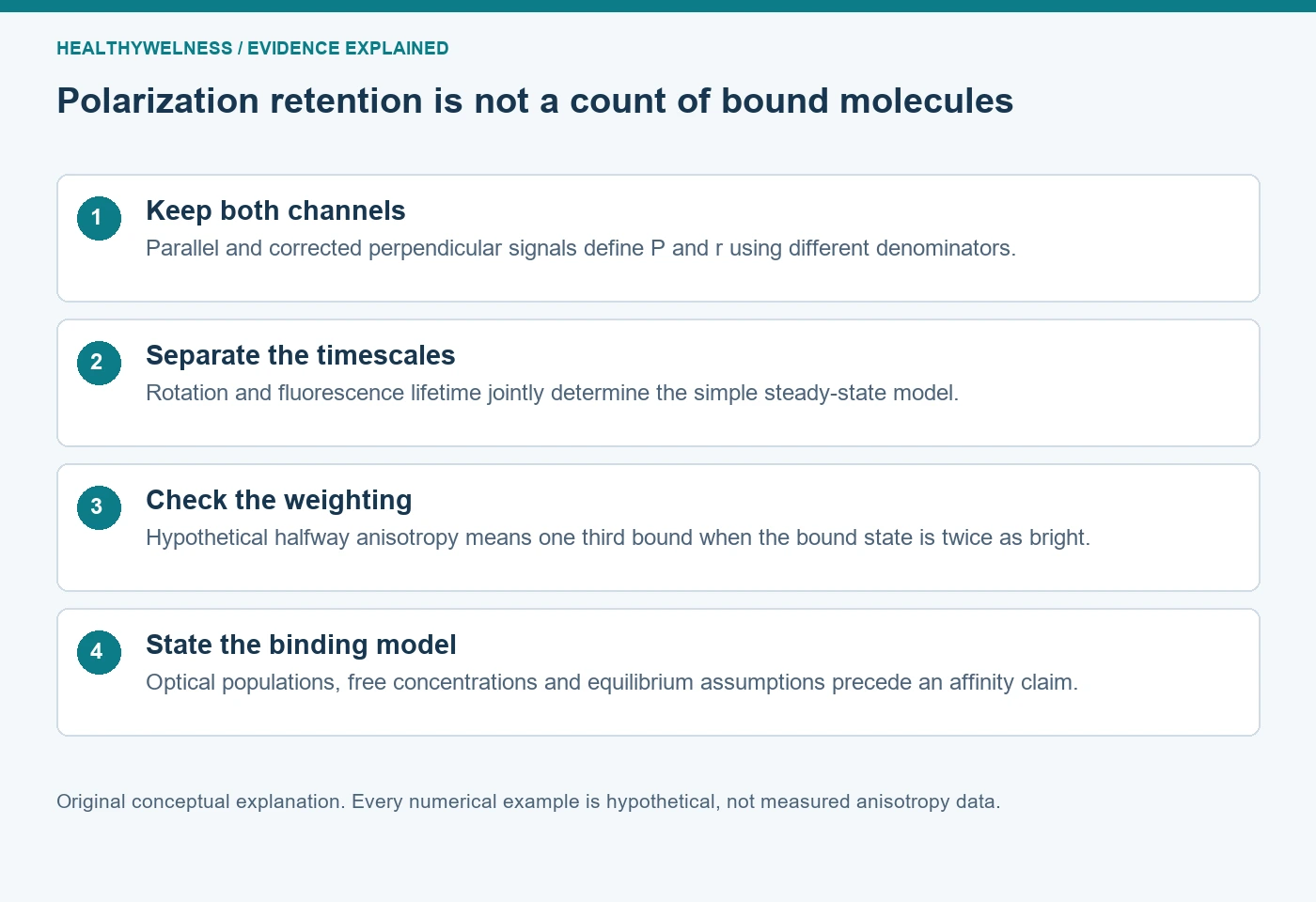
Cover and evidence map: original conceptual editorial schematics, not measured results, exact molecular structures, or photographs of HealthyWelness facilities.
Sources
- Thermo Fisher Scientific. Molecular Probes Handbook, Fluorescence Polarization (FP), Note 1.4. First-party technical guidance.
- Wei AP, Herron JN. Use of synthetic peptides as tracer antigens in fluorescence polarization immunoassays of high molecular weight analytes. Anal Chem. 1993. PMID8297026.
- Rossi AM, Taylor CW. Analysis of protein-ligand interactions by fluorescence polarization. Nat Protoc. 2011. PMID21372817.