Z-Prime Factor in Peptide Assays: Signal Window Limits
Understand Z-prime in peptide research assays, why signal-to-background misses variability, how to check calculations and what control separation means.


The Z′-factor summarizes separation between two assay-control populations relative to their variability. It helps assess whether an assay has a usable measurement window under specified conditions. A high signal-to-background ratio alone does not establish that separation, and a favorable Z′ does not prove peptide identity, target selectivity or biological relevance.
- Z′ combines the difference between control means with the spread of both control populations.
- Signal-to-background compares levels and can conceal large variability.
- A screening-quality metric is not a statistical significance test for a candidate peptide.
- Every numerical assay below is an invented teaching example, not a commercial-material measurement.
The control window must be separated from its noise
Imagine an assay in which the high-response control has a mean signal much larger than the low-response control. That sounds promising, but the two means do not show how widely individual readings vary. If the spread is large relative to their separation, one measured value may be difficult to classify reliably.
Zhang, Chung and Oldenburg introduced the Z-factor framework for high-throughput screening in 1999. Their original abstract defines a dimensionless screening-window characteristic that reflects both dynamic range and measurement variation. The abstract establishes the purpose of the metric; the detailed calculations used here are supported by the first-party guidance discussed below. [1]
The conventional control-based expression is Z′ = 1 − 3(σH + σL)/|μH − μL|. The symbols μ represent control means and σ their standard deviations. In practice, sample means and sample standard deviations estimate these quantities. Both control populations matter: an unstable low signal can damage separation even when the high control is precise.
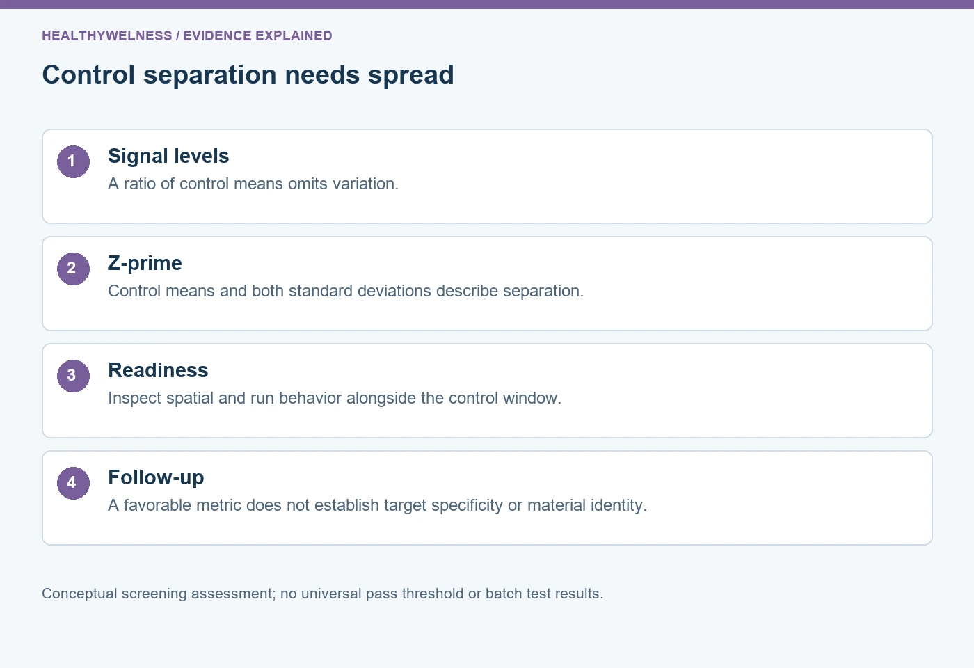
| Measure | Inputs | Does not establish |
|---|---|---|
| Signal/background | Defined signal levels | Control variability |
| Control range | Difference of means | Precision around means |
| Z′-factor | Means and both SDs | Target specificity |
| Candidate response | Test-condition signal | Assay-wide readiness |
Same signal ratio, different usable separation
Consider two invented assay settings. Each has a high-control mean of 1,000 detector units and a low-control mean of 100 units. Under a simple high-mean/low-mean definition, each therefore has a signal-to-background ratio of ten. The control range is 900 units in both settings.
In setting A, the high-control SD is 30 and the low-control SD is 10. The calculation is Z′ = 1 − 3(30 + 10)/900 = approximately 0.867. In setting B, the means stay unchanged but the SDs are 180 and 90. Its Z′ is 1 − 3(180 + 90)/900 = 0.100.
The signal ratio did not change; the spread did. The first setting has a much larger remaining separation relative to its range under this metric. No peptide became more potent or selective in this arithmetic. These are descriptions of stipulated control distributions, not pharmacological rankings or measured performance claims.
GraphPad’s calculation guide explains the separation-band interpretation: compare the distance remaining after three-SD margins around the controls with the distance between their means. This provides an intuitive way to read the formula without treating the ratio of means as a complete quality assessment. [2]
What do zero, positive and negative values mean?
When the conventional Z′ is zero, the mean separation equals three times the sum of the two SDs. A positive value means those chosen margins leave a gap. A negative value means the margins overlap. Negative Z′ is mathematically possible; it is not a missing value and should not silently be replaced by zero.
The three-SD choice is a convention in this metric, not a universal law of biological classification. Interpreting the margins as tail probabilities requires distributional assumptions. A skewed distribution, a mixture of states or occasional gross failures cannot be fully characterized by its mean and SD alone. Inspect the observations as well as calculating the summary.
With a nonzero mean difference and nonnegative SDs, the conventional expression cannot exceed one. If the control means are equal, the denominator is zero and the value is undefined. A computed value above one should trigger a check of signs, formulas and input definitions. It is not evidence for an exceptionally powerful assay.
A single cutoff also needs context. GraphPad describes the familiar 0.5-to-one range as excellent for screening. The Assay Guidance Manual’s HTS validation chapter uses Z′ ≥ 0.4 within a larger set of specified acceptance criteria. Those differences are a reason to state the framework being used, rather than declaring that one number universally validates every assay. [3]
Control selection determines what the metric describes
In common terminology, Z′ is calculated from positive and negative assay controls, whereas Z can involve a test-sample population and a control. Labels are sometimes used loosely, so report the formula and populations explicitly. The prime mark cannot rescue an ambiguous methods section.
A high and low control should represent relevant states of the assay. A maximum instrument signal that bypasses the biological or chemical measurement process may demonstrate detector range without testing variation in the complete assay. Similarly, controls prepared in a different matrix may fail to represent the variability encountered by study samples.
The direction of the response need not determine which condition is called positive. In an inhibition assay, the biologically positive control may generate the lower detector signal. Using high and low labels for the algebra avoids confusing biological direction with numerical magnitude. Keep the actual biological control identities visible alongside those labels.
- Identify the high- and low-signal conditions.
- State their relation to the intended assay process.
- Specify whether the values represent individual wells or summaries.
- Retain the plate, run and control identifiers used in calculation.
Technical aggregation can change the apparent quality
Suppose the intended screen uses one well for each test condition. Computing a metric from averages of many repeated control wells can make the control distribution look narrower than the single-well observations the screen will actually use. The apparent improvement may come from aggregation rather than a change in the production assay.
The Assay Guidance Manual explicitly considers the number of replicates used in the production format when describing signal-window calculations. The practical principle is to match the assessment to the measurement format it is supposed to characterize. A summary based on replicate averages should be labelled as such rather than compared uncritically with a single-well Z′.
More control wells improve information about means and spread; they do not make an individual well’s variability disappear. Nor should the SDs in the formula be casually replaced by SEMs. That substitution changes the quantity and can make the metric improve merely because more controls were collected. The SD, SEM and confidence-interval guide explains why those uncertainty measures serve different purposes.
A global number can hide an unfavorable plate pattern
Even separated overall control distributions can coexist with spatial drift, edge effects or day-to-day shifts that matter to the intended comparisons. Controls concentrated in one region may not reflect the experience of samples elsewhere. A summary statistic cannot establish that every location and run performs similarly.
The HTS validation guidance pairs signal-separation assessment with spatial uniformity and inter-plate and inter-day evaluation. Its structure is the important lesson: Z′ is one component of assessment. It does not replace inspection of raw plate patterns or evidence that intermediate responses can be measured consistently.
A screen designed to distinguish modest responses needs information about that region, not only the strongest possible high control. A wide extreme-control gap can coexist with poor discrimination among intermediate conditions. Interpret suitability against the actual research decision and preserve the relevant performance observations.
A favorable window does not identify a hit’s mechanism
A compound can alter fluorescence, interfere with a reporter or affect a process outside the proposed target while the controls remain well separated. A favorable Z′ therefore supports an operational statement about the control window, not a molecular conclusion about an individual candidate. Follow-up evidence should address the candidate’s alternative explanations.
The orthogonal-assay and counterscreen guide distinguishes independent measurement principles from tests for specific artifacts. Those experiments answer questions that a control-separation metric was never designed to resolve. A screening threshold is also separate from a statistical significance test, effect size or selectivity measurement.
Finally, an assay metric does not authenticate the tested material. The COA lookup provides a route to available analytical documentation. Neither a certificate nor Z′ independently establishes the complete evidence chain from molecular identity to a particular functional interpretation.
Frequently asked questions
Is a tenfold signal-to-background ratio enough?
No. It describes a ratio under a stated definition but omits the variability of the two populations. The invented example produces the same ratio with very different Z′ values.
Can Z′ be negative?
Yes. Negative values arise when three times the sum of control SDs exceeds the difference between control means. They should be reported and investigated rather than truncated to zero.
Is Z′ the same as a z score?
No. A z score expresses a value’s distance from a mean in SD units. Z′ characterizes separation between two assay-control populations.
Should SEM replace SD in the formula?
Not in the conventional control-distribution expression. SEM describes precision of an estimated mean. Substituting it changes the metric and can obscure variability relevant to individual screening measurements.
Does Z′ above 0.5 prove a peptide is active?
No. It concerns the specified control populations. A candidate response needs its own comparison, uncertainty assessment and follow-up interpretation; target-specific activity requires additional evidence.
Related reading
Continue with controls and experimental units for the role of comparators. The references below explain the screening metric, while the linked articles address distinct questions about evidence.
References
- Zhang JH, Chung TD, Oldenburg KR. A Simple Statistical Parameter for Use in Evaluation and Validation of High Throughput Screening Assays. Journal of Biomolecular Screening. 1999;4(2):67–73. PMID: 10838414. Original research; abstract verified.
- GraphPad Software. Calculating a Z-factor to assess the quality of a screening assay. FAQ 1153. First-party technical guidance.
- Iversen PW, et al. HTS Assay Validation. Assay Guidance Manual. NCATS guidance, signal separation and plate assessment.
Cover and evidence map: original conceptual editorial schematics, not measured results, exact molecular structures, or photographs of HealthyWelness facilities.