Endpoint vs Time-Course Peptide Assays: Reading Time
Compare endpoint and time-course peptide research assays: peak response, initial rate, response AUC, timing and the limits of a stable measured signal.

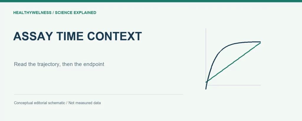
An endpoint assay measures a response at a specified time; a time-course assay records how that response develops. The two designs can answer different questions even in the same peptide experiment. A final value does not reveal the route taken to reach it, and a time course requires a clearly defined summary rather than an automatic claim of greater activity.
- Endpoint magnitude, peak response, initial rate and area under a response curve are different quantities.
- A stable measured signal can represent balanced production and loss rather than molecular equilibrium.
- Repeated readings of one well remain measurements of the same experimental unit.
- The invented trajectories below illustrate interpretation, not measured peptide behavior.
The clock is part of the endpoint definition
A signal reported as “response after exposure” is incomplete without the exposure interval and acquisition timing. Did the clock start when material was added, when mixing finished, or when the instrument began reading? Were wells read simultaneously or sequentially? Such differences can matter when the response changes quickly.
A fixed endpoint can be entirely appropriate when the research question concerns that defined time. It can also be efficient and reproducible. The limitation appears when one value is asked to establish onset, peak, duration or recovery without observations addressing those features. Identical endpoints are compatible with many different trajectories.
The Assay Guidance Manual’s GPCR-characterization chapter distinguishes transient, cumulative and sustained readouts. It explains how binding kinetics can influence measured responses and why real-time or time-lapse measurements provide additional information. This guidance concerns assay interpretation, not a universal optimal incubation period for research peptides. [1]
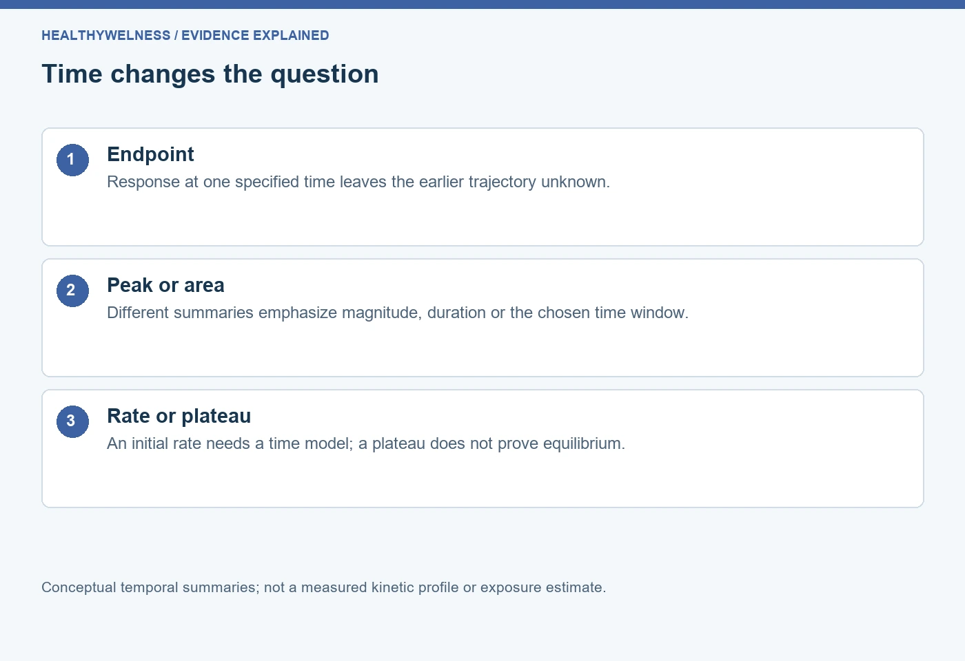
| Quantity | Question answered | Important boundary |
|---|---|---|
| Fixed endpoint | Response at chosen time | Earlier history hidden |
| Observed peak | Largest sampled response | Sampling can miss peak |
| Initial rate | Early response change/time | Needs suitable time model |
| Response AUC | Accumulated response/time | Depends on time window |
| Late plateau | Stable observed response | Not proof of equilibrium |
How can the apparent ranking reverse with time?
Consider invented baseline-corrected detector signals from two conditions, A and B. At 0, 2, 6 and 10 minutes, A has signals of 0, 80, 40 and 20 units, while B has 0, 20, 50 and 60 units. These are deliberately chosen teaching values. They are not measurements, recommendations or kinetic parameters for a named compound.
At two minutes A has four times B’s signal. At ten minutes B has three times A’s signal. Neither comparison contains an arithmetic error. They answer different temporal questions. Saying simply that one condition “produced the larger response” would conceal the observation time that determines the statement.
The largest sampled response is 80 for A and 60 for B. However, the actual continuous-time peaks remain unknown between measurements. A curve drawn through these points is a visualization choice; it does not prove that the process changed linearly between them or that the true peak occurred exactly when it was sampled.
Suppose the research question instead concerns the trapezoidal area from zero to ten minutes. Using the stipulated points, A gives 80 + 240 + 120 = 440 response-unit minutes; B gives 20 + 140 + 220 = 380. The area ranking follows A, whereas the final endpoint ranking follows B. This difference shows why the desired summary must be named before interpreting a comparison.
- Early endpoint: emphasizes the response present early.
- Late endpoint: emphasizes the response remaining later.
- Peak: emphasizes the largest observed excursion.
- Area: combines magnitude and duration within a specified interval.
Response AUC is not an exposure measurement
The units of the area calculation matter. Integrating a detector response over minutes gives response-unit minutes. It does not automatically give peptide concentration multiplied by time, molecular residence time or an amount of intact material. Those quantities require different observations or a supported measurement model.
AUC also depends on baseline definition, start and stop times, sampling density and numerical integration. Extending the window can change a comparison if one condition persists longer. Subtracting an unsuitable baseline can create negative areas or change relative areas. The problem is interpretive before it is computational.
For a comparison across papers, first reconcile what was integrated. Calcium fluorescence, reporter expression and measured parent-peptide concentration are different axes. Even matching time units cannot make their areas interchangeable. A useful extraction sheet preserves response units and integration bounds instead of collecting every quantity labelled AUC into one column.
An initial rate needs more than division by elapsed time
In the invented example, A rises by 80 units over the first two minutes, giving an interval-average change of 40 units per minute. That is not necessarily the instantaneous rate at time zero. There may have been an unobserved lag or an early peak. The data determine which distinction can be supported.
Hoare and colleagues developed a GPCR signaling analysis framework that treats kinetic profiles explicitly, including rise-and-fall and sustained-response shapes. Their approach can estimate an initial signaling rate by fitting a whole trajectory under its stated assumptions. The result is a model-based kinetic quantity rather than an endpoint divided by incubation time. [2]
In separate original research, Hoare and colleagues used a fluorescent biosensor platform for arrestin recruitment at angiotensin AT1 and vasopressin V2 receptors, combined with kinetic analysis. That experimental setting illustrates a reason to acquire trajectories: it permits questions about response development that one final reading cannot resolve. It does not validate the same model for every fluorescent peptide experiment. [3]
The related enzyme-kinetics guide explains initial reaction rates in substrate conversion. Here the broader issue is selecting a temporal response quantity, including cellular signals that can rise, decline or persist.
A plateau does not prove the system has equilibrated
A constant signal can have several explanations. In a dynamic system, ongoing signal production may balance signal loss. A detector may saturate. A cumulative assay may exhaust a reagent. Several changing processes may offset one another. A flat observed trace alone does not distinguish those possibilities.
Hoare and colleagues distinguish an approach to a plateau from a rise followed by decline to a sustained level. Those shapes carry different information despite potentially sharing the same late reading. Their analysis separates empirical curve shapes from mechanistic explanations, which require knowledge of the system. Do not infer a unique molecular pathway from visual resemblance alone.
Equilibrium binding and cellular steady response are also different concepts. A steady signal does not establish that free ligand, receptor occupancy and downstream signaling have all reached the same kind of equilibrium. Report what became approximately stable over the observed interval, with the measurement and resolution stated.
Repeated measurement introduces its own dependencies
A trace containing sixty readings from one well has sixty time observations, not sixty independent biological preparations. Successive readings share the sample, its preparation history and often correlated measurement behavior. Averaging or modelling a trace should preserve that dependence rather than manufacturing a larger independent sample count.
Some time-course methods repeatedly observe the same preparation; others require separate samples because measurement consumes or alters the material. These designs have different dependence structures. The label “time course” is insufficient to identify the experimental unit. Record whether each time point comes from the same well, a separate aliquot, or an independent preparation.
Acquisition itself may matter. Mixing delay can conceal fast onset, sequential plate reading can offset effective time across wells, and repeated illumination can change an optical readout. These are alternatives to investigate when relevant to the method, not assumed explanations for every unusual trajectory. Include suitable controls and inspect whether timing was comparable across conditions.
Specify the analysis window before choosing a favorable result
If several endpoints, peaks, areas and rates are available, choosing whichever gives the most striking contrast after inspecting the curves changes the analysis question. A useful plan identifies the main temporal quantity and window, then distinguishes exploratory summaries. Unexpected behavior can justify follow-up without rewriting the original comparison as though it had been planned.
For curve fitting, state the equation, fitting interval, baseline treatment, constraints and uncertainty. A more complicated equation can fit fluctuations without establishing more molecular detail. Conversely, forcing a monotonic model onto a clear rise-and-fall trace can hide the feature the experiment was designed to investigate.
Timing cannot replace material identification. The COA lookup is a route to available analytical documentation, while temporal assay data describe response under stated conditions. Neither layer independently establishes the other, and this article supplies no batch-specific testing claims.
Frequently asked questions
Is a time-course assay always better than an endpoint assay?
No. It provides additional temporal observations but also requires suitable acquisition and analysis. An endpoint can answer a defined time-specific question adequately; it cannot reconstruct an unmeasured trajectory.
Can two peptides have the same endpoint but different kinetics?
Yes. Different onset, peaks, declines and sustained levels can converge to the same reading at one time. Additional time observations are needed to distinguish those histories.
Is the largest sampled point the true peak?
It is the observed peak under the sampling scheme. A faster excursion between readings may have been missed, so the continuous-time maximum can remain uncertain.
Does a flat response mean equilibrium binding?
No. A stable readout can reflect dynamic balance or limitations of measurement. Equilibrium binding requires evidence appropriate to binding, rather than a flat downstream signal alone.
Can response AUC be compared across different time windows?
The windows must remain explicit. Different bounds describe different accumulated responses, and a ranking may change as the window extends. Matching the window is necessary but not sufficient for comparability.
Related reading
Continue with affinity and functional potency, response normalization and references, and experimental units and controls.
References
- Assay Guidance Manual. Pharmacological Characterization of GPCR Agonists, Antagonists, Allosteric Modulators and Biased Ligands from HTS Hits to Lead Optimization. NCATS technical guidance.
- Hoare SRJ, et al. Analyzing kinetic signaling data for G-protein-coupled receptors. Scientific Reports. 2020;10:12263. PMID: 32704081. Original research.
- Hoare SRJ, et al. A kinetic method for measuring agonist efficacy and ligand bias using high resolution biosensors and a kinetic data analysis framework. Scientific Reports. 2020;10:1766. PMID: 32019973. Original research.
Cover and evidence map: original conceptual editorial schematics, not measured results, exact molecular structures, or photographs of HealthyWelness facilities.
Sources
- Assay Guidance Manual: Pharmacological Characterization of GPCR Agonists, Antagonists, Allosteric Modulators and Biased Ligands
- Hoare et al. Analyzing kinetic signaling data for G-protein-coupled receptors (2020)
- Hoare et al. A kinetic method for measuring agonist efficacy and ligand bias using high resolution biosensors and a kinetic data analysis framework (2020)